Ruby Benchmarking & Big O Notation
The Ruby Benchmark library helps us to measure how long it takes for a block of code to run. Similar to when you subtract starting time and ending time in other languages such as Java.
I was doing some Big O Notation reviewing with Ruby the other day and did some common algorithm implementations for each of the most common Big O notations, just for fun.
Using Benchmark
To start benchmarking our code, we simply need to require benchmark and use the methods provided by the Benchmark module. For me, the most practical way is to use Benchmark#bm method, where we pass a block of code we want to measure:
require 'benchmark'

Benchmark.bm do |x|
  x.report do
    # our code here
  end

end
Inside the block we are using the report method of the block's variable, which will basically do a separate benchmark for each report.
However, we can improve this even more by adding a label to report and a label width to bm:
require 'benchmark'

Benchmark.bm(20) do |x|
  x.report("my_algorithm") do
    # our code here
  end
end
Let's see it in action with some common algorithms.
What is Big O Notation?
Big O notation is a special notation that measures how well a computer algorithm scales, as the amount of data involved increases (becomes closer to infinity). It is not necessarily a measurement of speed, but of how well the algorithm scales.
The following are some of the most common Big O notations, with algorithms and benchmarks.
O(1)
O(1) represents constant time. This means that the algorithm will execute in the same amount of time regardless of the amount of data or input. This is an ideal time complexity, and in algorithms with a time complexity greater than O(1) it can still be achieved by using techniques such as memoization.
An example of O(1) would be simply adding an element to an array. The size of the array won't matter when simply adding a new element at the end:
Benchmark.bm(10) do |x|
  a = [1, 2, 3, 4, 5]
  x.report("add_element") { a.push(6) }

  a = (1..9_000_000).to_a
  x.report("add_element") { a.push(6) }
end
The benchmark results are:
                 user     system      total        real
add_element  0.000000   0.000000   0.000000 (  0.000003)
add_element  0.000000   0.000000   0.000000 (  0.000012)
We can clearly see that there is practically no difference between adding to the 5 element array and adding to the 9 million element array.
O(n)
O(n) represents linear time. This means that the time to complete the algorithm is proportional to the amount of data. A good example of this is linear search, simply because looking for an element in a 9 million size array will take a lot longer than looking in a 10 size element array.
# O(N)
def linear_search(array, value)
  array.each { |i| return i if i == value }
end

Benchmark.bm(50) do |x|
  x.report("linear_search(1,000)") { linear_search(1000) }
  x.report("linear_search(10,000,000)") { linear_search(10_000_000) }
end
The benchmark results are:
                                                         user     system      total        real
linear_search(1,000)                                 0.000000   0.000000   0.000000 (  0.000102)
linear_search(10,000,000)                             0.700000   0.000000   0.700000 (  0.722858)
Still pretty fast, but the difference is very noticeable.
O(n^2)
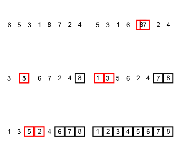
O(n^2) indicates that the amount to complete will be proportional to the square of the amount of data. This usually happens with algorithms that have nested loops. A good example of this notation is the bubble sort algorithm.

Here is a simple implementation in Ruby, with its corresponding benchmarks:
# O(N^2)
def bubble_sort(array)
  n = array.length

  loop do
    swapped = false

    (n-1).times do |i|
      if array[i] > array[i+1]
        array[i], array[i+1] = array[i+1], array[i]
        swapped = true
      end
    end
    break if not swapped
  end

  array
end

Benchmark.bm(50) do |x|
  x.report("bubble_sort([1..10])") { bubble_sort((1..10).to_a.shuffle) }
  x.report("bubble_sort([1..10,000])") { bubble_sort((1..10_000).to_a.shuffle) }
end
The benchmark results are:
                                                         user     system      total        real
bubble_sort([1..10])                                 0.000000   0.000000   0.000000 (  0.000039)
bubble_sort([1..10,000])                            13.990000   0.010000  14.000000 ( 14.028724)
Now we are starting to see a lot more difference. This is because we initially have to loop through the whole array, and for each element in the iteration, we loop through the whole array again. Hence resulting in: O(n) x O(n) = O(n^2).
When the amount of input is relatively small, O(n^2) algorithm's bad performance will not be that obvious. But as the input size grows, it will become more evident, and that is why O(n^2) algorithms are generally avoided for big inputs.
O(log n)
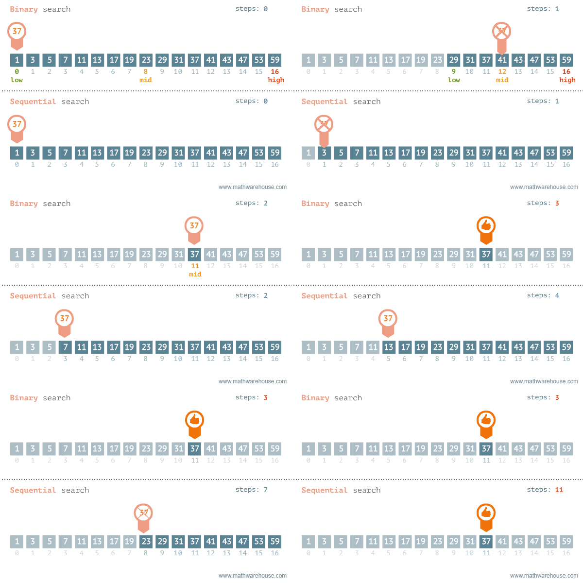
O(log n) is a much more efficient algorithm. This is because the input used is decreased by around 50% each time through the algorithm. These kind of algorithms are very fast and efficient because increases in the amount of data have little to no effect at some point early on because the amount of data is half each time.
A good example of an O(log n) algorithm is the binary search algorithm:

In Ruby, we can implement a binary search in the following way (NOTE: The array must be initially sorted for the algorithm to work.):
# O( log N )
def binary_search(array, element, low=0, high=array.length-1)
  return nil if high < low

  mid = ( low + high ) / 2

  if array[mid] > element
    return binary_search(array, element, low, mid - 1)
  elsif array[mid] < element
    return binary_search(array, element, mid + 1, high)
  else
    return mid
  end
end

Benchmark.bm(50) do |x|
  x.report("binary_search([1..10])") { binary_search((1..10).to_a, 4) }
  x.report("binary_search([1..5,000,000])") { binary_search((1..5_000_000).to_a, 4_999_999) }
end
The benchmark results are:
                                                         user     system      total        real
binary_search([1..10])                               0.000000   0.000000   0.000000 (  0.000011)
binary_search([1..5,000,000])                        0.190000   0.000000   0.190000 (  0.192921)
It is clearly obvious that the performance difference of the algorithm with an array of size 10 compared to that of with an array of size 5,000,000 is almost non-existent, even when using a “worst case” (in this case, the element before the last one).
O(n log n)
In sorting algorithms, a time complexity of at least O(n) is unavoidable (at least in theory). This is because we have to look at each element in the array at least once in order to properly sort it. At the same time, an order of O(n^2) is to be avoided.
O(n log n) sorting algorithms are more efficient because values are only compared once, instead of being compared to each other repeatedly. This means that each comparison will reduce the possible final sorted list in half.
In other words, we can calculate the number of comparisons like this:
number_comparisons = log(n!)
      log(n) + log(n-1) + ... + log(1)
      nlog(n)
      log n + log (n-1) + ... + log (n/2)
      n/2 * log (n/2)
  =>  nlog(n)
A good example of a O(n log n) algorithm is the quick sort algorithm:

In Ruby, we can implement Quicksort like this:
# O( N log N )
def quick_sort(array)
  return array if array.length <= 1

  pivot = array[0]

  less, greatereq = array[1..-1].partition { |x| x < pivot }
  quick_sort(less) + [pivot] + quick_sort(greatereq)
end

Benchmark.bm(50) do |x|
  x.report("quick_sort([1..20])") { quick_sort((1..20).to_a.shuffle) }
  x.report("quick_sort([1..400,000])") { quick_sort((1..400_000).to_a.shuffle) }
end
Notice how multiple assignment and the partition method from Enumerable is used. This method will return two arrays: the first array will contain elements for which the block evaluates to true, and the second one containing the rest.
The benchmark yields the following results:
                                                         user     system      total        real
quick_sort([1..20])                                  0.000000   0.000000   0.000000 (  0.000048)
quick_sort([1..400,000])                             1.400000   0.020000   1.420000 (  1.430095)
Closing Thoughts
Even though those are the most common Big O time complexity notations, there are even more complicated complexities (lol?) out there.
Moreover, there are also other asymptotic notations that use different symbols to describe different kinds of bounds. I hope to cover these sometime in the future.